

The INDEX function returns a specific value from a one-dimensional or two-dimensional range.
The MATCH function returns the relative position number of an item.
The INDEX function actually returns the value in the cell, not the position.
Let’s examine the INDEX function syntax below
=INDEX (array, row_num, [column_num])
- The array (First argument) is the range that has the value you wish to return
- The row_num (Second argument) is the row number within the range that contains the value to return.
- The [column_num] (Third argument) is the optional column number within the range that contains the value to return. This can be used to perform either one- or two-dimensional lookups.
Note this while inputting the INDEX formula – You define a lookup range, called the array, in the first argument. Then you tell Excel how many rows down to go via the second argument. Then, optionally, you tell Excel to go a certain number of columns across via the third argument.
You can watch the video option of the tutorial below
SCENARIO 1
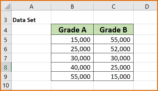
We will be working with the data set below to return a specific value from a two-dimensional range
Input the formula below into cell E8
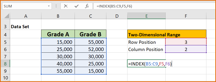
The result of the formula below shows that at the point of intersection of row 3 (cell B7) and column 2 (cell C7) cell E8 returns a value of 30,000 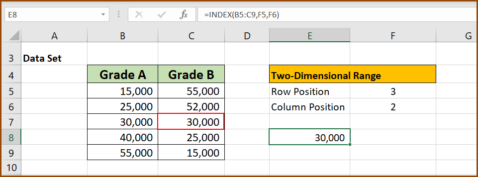
SCENARIO 2
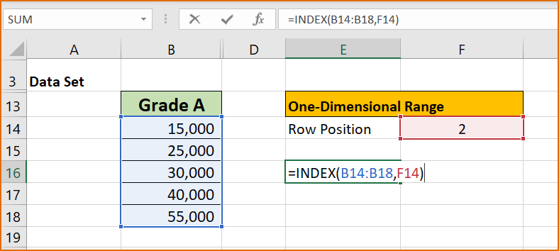
Here we will be working with a one-dimensional range data set
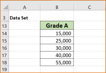
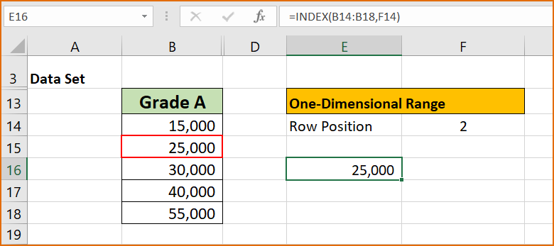
Input the formula below in cell E16
The formula returns a value of 25,000 in cell E16. This value is found in row 2 (cell B15) of the range B14:B18
Here is the link to download the workbook so you can practice along.
Hey!
Did you get value from this tutorial?
I will love to know how well you now understand the INDEX function after reading through and working along.
Kindly use the comment section to send your feedback as this will help serve you better.
Do well to share this insightful tutorial with others.
Thank you!