

The MATCH function returns the position of a value in a given range.
Let’s examine the function syntax
=MATCH(lookup_value, lookup_array, [match_type])
lookup_value is the first argument in the Function syntax. It can be a cell reference, value or text string.
lookup_array is the second argument in the function syntax. This is the cell range to be looked up.
[match_type] is the last function argument and allows the user to select the match type.
Note:
- If a match type 1 is specified, the function returns the largest value that is less than or equal to the lookup value. This option requires the cell range to be sorted in ascending order.
- A match type 0 returns a value if an exact match of the lookup value can be found in the lookup cell range.
- If an exact match of the lookup value cannot be found, a #N/A error is returned.
- If a match type -1 is specified, the MATCH function returns the smallest value in the lookup cell range that is greater than or equal to the lookup value. This option requires the lookup cell range to be sorted in descending order
You can watch the video lesson here as you read through
Download the workbook so you can work along
Let me show you how this works using different scenarios for better understanding.
Here is the data set used in each of the scenarios for better illustration

Data Set A is arranged in ascending order as this is required when a match type 1 is used in the third or last argument.
Data Set B is arranged in descending order as this is required when a match type -1 is used in the third or last argument.
SCENARIO 1
Using a match type 1, let’s get the position of the value in cell F6 within the range A5:A9, by inputting the formula below in cell G6
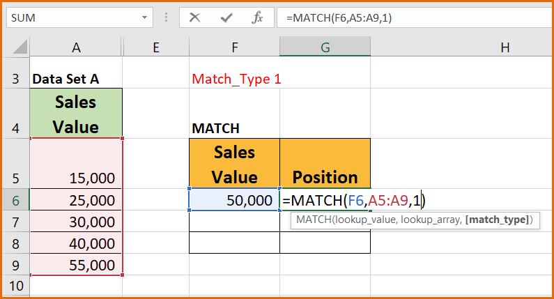
The result of the formula in cell G6 below shows that the sales value in cell F6 is in the 4th position based on the lookup cell range (A5:A6) selected.

Explanation:
- The lookup value that has been specified in cell F6 has a value of 50,000. The function returns a value of 4 because 40,000 is the largest value in the lookup cell range (A5:A9) that is less than or equal to 50,000 and it’s in the 4th position of the lookup cell range.
Note:
- This option (match type 1) requires the cell range (A5:A9) to be sorted in ascending order.
SCENARIO 2
Let’s consider another scenario using a match type 0
Input the formula below into cell J6

The result of the formula in cell J6 below shows that the sales value in cell I6 is in the 4th position based on the lookup cell range (A5:A9) selected.

Explanation:
- The MATCH function with match type 0 only returns a value if an exact match of the lookup value can be found in the lookup cell range. The lookup value that has been specified in cell I6 has a value of 40,000. The function returns a value of 4 because 40,000 is the 4th value in the lookup cell range (A5:A9).
Note:
- If an exact match of the lookup value cannot be found, a #N/A error is returned by the function.
- The range does not need to be arranged either in ascending or descending order.
SCENARIO 3
Let’s consider another example using the match type -1
Input the formula in cell M6 below

The result of the formula in cell M6 below shows that the sales value in cell L6 is in the 2nd position based on the lookup cell range (C5:C9) selected.

Explanation:
- The lookup value that has been specified in cell L6 has a value of 50,000. The function returns a value of 2 because 52,000 is the largest value in the lookup cell range that is less than or equal to 50,000 and it’s in the 2nd position of the lookup cell range.
Note:
- This option (match type -1) requires the cell range (C5:C9) to be sorted in descending order.
Hey!
Did you get value from this blog post tutorial?
I will love to know how well you now understand the MATCH function after reading through and working along.
Kindly use the comment section to send your feedback as this will help serve you better.
Do well to share this insightful tutorial with others.
Thank you!